以AlexNet为例分析pytorch

以AlexNet分析,对比pytorch和TensorFlow

背景

  • 先前的深度学习都是使用的TensorFlow框架的,这是因为TensorFlow占领市场较早,生态社区建立得早,但是不得不说,tf仍然是公认的难用。
  • 使用pytorch,在pytorch官网上稍微花点时间,就可以部署好。比原本从python到C++部署TensorFlow的时间缩短好几倍。
  • 另外pytorch也是公认的易于上手,相比TensorFlow这种反人类的设计,可以说非常人性化了
  • 这篇博客就是以AlexNet为例,一步步分析网络。再对比TensorFlow和pytorch的不同,也算是是为了学习。

分析网络

先上个网络结构图,这个图片上一篇博文里面已经放过了,基本表示了8层网络的结构
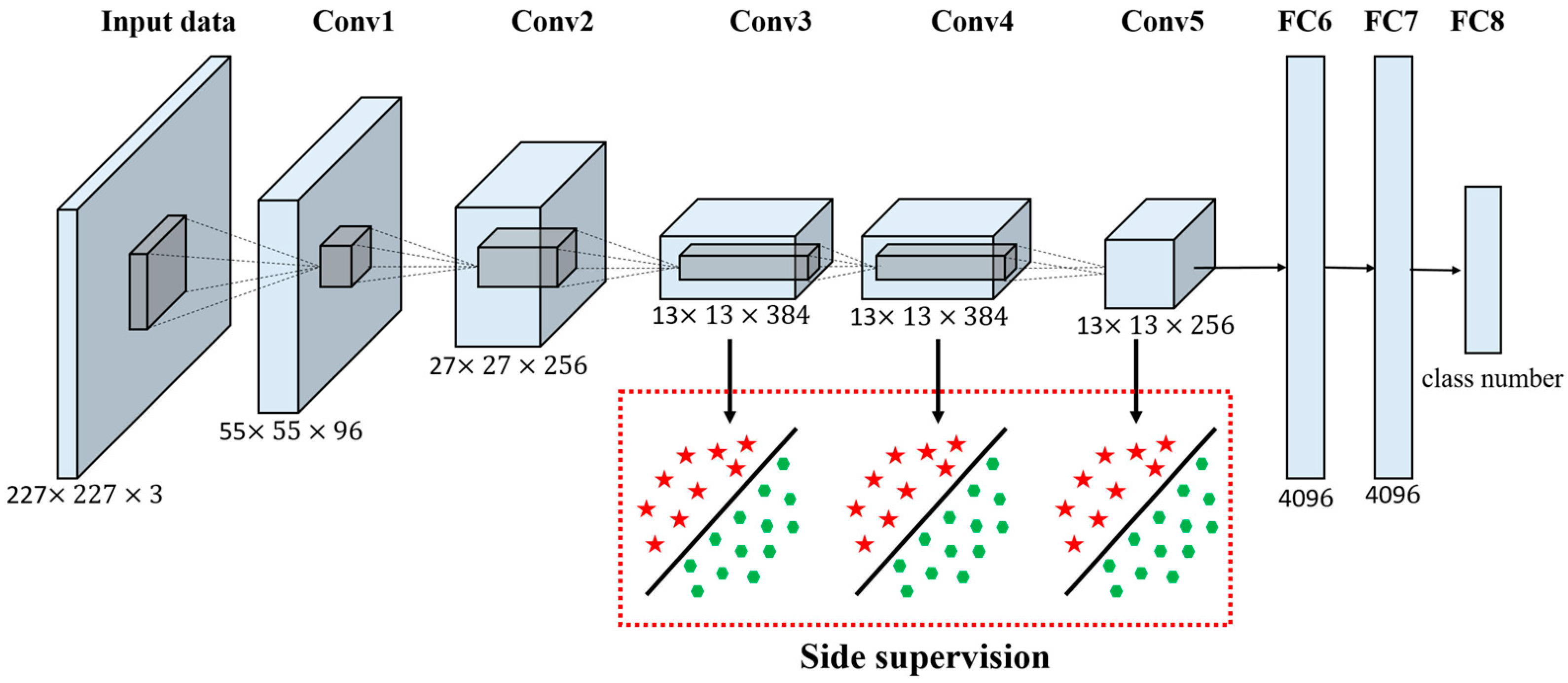

AlexNet

输入图片是227*227的RGB三通道图片,先后经过五个卷积层,和三个全连接层,得到输出。这里面五个卷积层:

  • 卷积层的作用就是提取信息,减维度。第二个卷积层为例,参数有:
    Conv_input卷积输入,
    Kernal_size卷积核大小,
    Kernal_nums卷积核数目,
    Stride步长
    Pad补丁
    Conv_output卷积输出
    假设输入是等高宽的,则输出就表示成:
    输出宽(高)=(输入的宽(高)-卷积核宽(高)+2*补丁)/ 步长+1
    输出通道数 = 卷积核数目

  • 池化层,暴力降维。以第一个池化层为例,参数有
    Pool_input池化输入
    Kernal_size卷积核大小
    Stride步长
    Pool_output卷积输出
    同样假设输入等宽高,输出计算:
    池化输出 = 宽(高)=(输入的宽(高)-卷积核宽(高))/ 步长+1

  • 全连接层


    全连接层没啥好说的,就是映射。下面就是AlexNet公认的几个贡献:

  1. ReLU作为激活函数
  2. Dropout避免模型过拟合
  3. 最大池化
  4. 提出LRN层
  5. GPU加速

TensorFlow下的AlexNet

代码使用来源:修炼之路

1
2
3
4
5
6
7
8
9
10
11
12
13
14
15
16
17
18
19
20
21
22
23
24
25
26
27
28
29
30
31
32
33
34
35
36
37
38
39
40
41
42
43
44
45
46
47
48
49
50
51
52
53
54
55
56
57
58
59
60
61
62
63
64
65
66
67
68
69
70
71
72
73
74
75
76
77
78
79
80
81
82
83
84
85
86
87
88
89
90
91
92
93
94
95
96
97
98
99
100
101
102
103
104
105
106
107
108
#第一层卷积层
with tf.name_scope("conv1") as scope:
#设置卷积核11×11,3通道,64个卷积核
kernel1 = tf.Variable(tf.truncated_normal([11,11,3,64],mean=0,stddev=0.1,
dtype=tf.float32),name="weights")
#卷积,卷积的横向步长和竖向步长都为4
conv = tf.nn.conv2d(images,kernel1,[1,4,4,1],padding="SAME")
#初始化偏置
biases = tf.Variable(tf.constant(0,shape=[64],dtype=tf.float32),trainable=True,name="biases")
bias = tf.nn.bias_add(conv,biases)
#RELU激活函数
conv1 = tf.nn.relu(bias,name=scope)
#输出该层的信息
print_tensor_info(conv1)
#统计参数
parameters += [kernel1,biases]
#lrn处理
lrn1 = tf.nn.lrn(conv1,4,bias=1,alpha=1e-3/9,beta=0.75,name="lrn1")
#最大池化
pool1 = tf.nn.max_pool(lrn1,ksize=[1,3,3,1],strides=[1,2,2,1],padding="VALID",name="pool1")
#输出该层信息
print_tensor_info(pool1)

#第二层卷积层
with tf.name_scope("conv2") as scope:
#初始化权重
kernel2 = tf.Variable(tf.truncated_normal([5,5,64,192],dtype=tf.float32,stddev=0.1)
,name="weights")
conv = tf.nn.conv2d(pool1,kernel2,[1,1,1,1],padding="SAME")
#初始化偏置
biases = tf.Variable(tf.constant(0,dtype=tf.float32,shape=[192])
,trainable=True,name="biases")
bias = tf.nn.bias_add(conv,biases)
#RELU激活
conv2 = tf.nn.relu(bias,name=scope)
print_tensor_info(conv2)
parameters += [kernel2,biases]
#LRN
lrn2 = tf.nn.lrn(conv2,4,1.0,alpha=1e-3/9,beta=0.75,name="lrn2")
#最大池化
pool2 = tf.nn.max_pool(lrn2,[1,3,3,1],[1,2,2,1],padding="VALID",name="pool2")
print_tensor_info(pool2)

#第三层卷积层
with tf.name_scope("conv3") as scope:
#初始化权重
kernel3 = tf.Variable(tf.truncated_normal([3,3,192,384],dtype=tf.float32,stddev=0.1)
,name="weights")
conv = tf.nn.conv2d(pool2,kernel3,strides=[1,1,1,1],padding="SAME")
biases = tf.Variable(tf.constant(0.0,shape=[384],dtype=tf.float32),trainable=True,name="biases")
bias = tf.nn.bias_add(conv,biases)
#RELU激活层
conv3 = tf.nn.relu(bias,name=scope)
parameters += [kernel3,biases]
print_tensor_info(conv3)

#第四层卷积层
with tf.name_scope("conv4") as scope:
#初始化权重
kernel4 = tf.Variable(tf.truncated_normal([3,3,384,256],stddev=0.1,dtype=tf.float32),
name="weights")
#卷积
conv = tf.nn.conv2d(conv3,kernel4,strides=[1,1,1,1],padding="SAME")
biases = tf.Variable(tf.constant(0.0,dtype=tf.float32,shape=[256]),trainable=True,name="biases")
bias = tf.nn.bias_add(conv,biases)
#RELU激活
conv4 = tf.nn.relu(bias,name=scope)
parameters += [kernel4,biases]
print_tensor_info(conv4)

#第五层卷积层
with tf.name_scope("conv5") as scope:
#初始化权重
kernel5 = tf.Variable(tf.truncated_normal([3,3,256,256],stddev=0.1,dtype=tf.float32),
name="weights")
conv = tf.nn.conv2d(conv4,kernel5,strides=[1,1,1,1],padding="SAME")
biases = tf.Variable(tf.constant(0.0,dtype=tf.float32,shape=[256]),name="biases")
bias = tf.nn.bias_add(conv,biases)
#REUL激活层
conv5 = tf.nn.relu(bias)
parameters += [kernel5,bias]
#最大池化
pool5 = tf.nn.max_pool(conv5,[1,3,3,1],[1,2,2,1],padding="VALID",name="pool5")
print_tensor_info(pool5)

#第六层全连接层
pool5 = tf.reshape(pool5,(-1,6*6*256))
weight6 = tf.Variable(tf.truncated_normal([6*6*256,4096],stddev=0.1,dtype=tf.float32),
name="weight6")
ful_bias1 = tf.Variable(tf.constant(0.0,dtype=tf.float32,shape=[4096]),name="ful_bias1")
ful_con1 = tf.nn.relu(tf.add(tf.matmul(pool5,weight6),ful_bias1))

#第七层第二层全连接层
weight7 = tf.Variable(tf.truncated_normal([4096,4096],stddev=0.1,dtype=tf.float32),
name="weight7")
ful_bias2 = tf.Variable(tf.constant(0.0,dtype=tf.float32,shape=[4096]),name="ful_bias2")
ful_con2 = tf.nn.relu(tf.add(tf.matmul(ful_con1,weight7),ful_bias2))
#
#第八层第三层全连接层
weight8 = tf.Variable(tf.truncated_normal([4096,1000],stddev=0.1,dtype=tf.float32),
name="weight8")
ful_bias3 = tf.Variable(tf.constant(0.0,dtype=tf.float32,shape=[1000]),name="ful_bias3")
ful_con3 = tf.nn.relu(tf.add(tf.matmul(ful_con2,weight8),ful_bias3))

#softmax层
weight9 = tf.Variable(tf.truncated_normal([1000,10],stddev=0.1),dtype=tf.float32,name="weight9")
bias9 = tf.Variable(tf.constant(0.0,shape=[10]),dtype=tf.float32,name="bias9")
output_softmax = tf.nn.softmax(tf.matmul(ful_con3,weight9)+bias9)

pytorch下的AlexNet

代码来源:sjtu_leexx

1
2
3
4
5
6
7
8
9
10
11
12
13
14
15
16
17
18
19
20
21
22
23
24
25
26
27
28
29
30
31
32
33
34
35
36
37
38
39
40
41
42
43
44
45
46
47
48
49
50
51
52
53
class BuildAlexNet(nn.Module):
def __init__(self, model_type, n_output):
super(BuildAlexNet, self).__init__()
self.model_type = model_type
if model_type == 'pre':
model = models.alexnet(pretrained=True)
self.features = model.features
fc1 = nn.Linear(9216, 4096)
fc1.bias = model.classifier[1].bias
fc1.weight = model.classifier[1].weight

fc2 = nn.Linear(4096, 4096)
fc2.bias = model.classifier[4].bias
fc2.weight = model.classifier[4].weight

self.classifier = nn.Sequential(
nn.Dropout(),
fc1,
nn.ReLU(inplace=True),
nn.Dropout(),
fc2,
nn.ReLU(inplace=True),
nn.Linear(4096, n_output))
#或者直接修改为
# model.classifier[6]==nn.Linear(4096,n_output)
# self.classifier = model.classifier
if model_type == 'new':
self.features = nn.Sequential(
nn.Conv2d(3, 64, 11, 4, 2),
nn.ReLU(inplace = True),
nn.MaxPool2d(3, 2, 0),
nn.Conv2d(64, 192, 5, 1, 2),
nn.ReLU(inplace=True),
nn.MaxPool2d(3, 2, 0),
nn.Conv2d(192, 384, 3, 1, 1),
nn.ReLU(inplace = True),
nn.Conv2d(384, 256, 3, 1, 1),
nn.ReLU(inplace=True),
nn.MaxPool2d(3, 2, 0))
self.classifier = nn.Sequential(
nn.Dropout(),
nn.Linear(9216, 4096),
nn.ReLU(inplace=True),
nn.Dropout(),
nn.Linear(4096, 4096),
nn.ReLU(inplace=True),
nn.Linear(4096, n_output))

def forward(self, x):
x = self.features(x)
x = x.view(x.size(0), -1)
out = self.classifier(x)
return out

直观比较

  • 直观感受就是pytorch比TensorFlow好多了。
  • 同时pytorch是有预训练数据的,可以用来迁移学习。
  • Tensorflow供给用户修改的参数实在太多了,细致到每一层的命名。而pytorch封装得很好,参数就少很多。最后结果就是使用起来,其实更方便。

代码上比较

用TensorFlow写一个卷积层,第二层为例:

1
2
3
4
5
6
7
8
9
10
11
12
13
14
15
16
17
18
19
#第二层卷积层
with tf.name_scope("conv2") as scope:
#初始化权重
kernel2 = tf.Variable(tf.truncated_normal([5,5,64,192],dtype=tf.float32,stddev=0.1)
,name="weights")
conv = tf.nn.conv2d(pool1,kernel2,[1,1,1,1],padding="SAME")
#初始化偏置
biases = tf.Variable(tf.constant(0,dtype=tf.float32,shape=[192])
,trainable=True,name="biases")
bias = tf.nn.bias_add(conv,biases)
#RELU激活
conv2 = tf.nn.relu(bias,name=scope)
print_tensor_info(conv2)
parameters += [kernel2,biases]
#LRN
lrn2 = tf.nn.lrn(conv2,4,1.0,alpha=1e-3/9,beta=0.75,name="lrn2")
#最大池化
pool2 = tf.nn.max_pool(lrn2,[1,3,3,1],[1,2,2,1],padding="VALID",name="pool2")
print_tensor_info(pool2)

  • 每层都命名,这可能对可视化调试有些帮助,但是在网络逐渐变深的现在意义不大。
  • 偏置和卷积核都用tf.Variable设置的变量,而且变量还是多,繁琐

同样用pytorch写第二个层,就可以是

1
2
3
nn.Conv2d(64, 192, 5, 1, 2),
nn.ReLU(inplace=True),
nn.MaxPool2d(3, 2, 0),

这写在nn.Sequential函数里面,会按序传播的。补一句解释:inplace为True,将会改变输入的数据 ,否则不会改变原输入,只会产生新的输出。是用于反向传播的。
最后说一句,pytorch做迁移学习是真方便